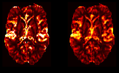
Fabber models for DSC-MRI¶

These models use the Fabber Bayesian model fitting framework [1] to implement a two models for Dynamic Susceptibility Contrast MRI (DSC-MRI).

If you are simply looking to process standard DSC data you should probably look instead at the Verbena tool which uses Fabber_DSC as its modelling implementation. This documentation provides a little more details on the model implementation for people who are interested in using the models directly.

Getting FABBER_DSC¶

The DSC models are included as part of FSL. Version 6.0.1 or later is strongly recommended - this documentation describes the version of the DSC models included in the current FSL release.

Models included¶

Two DSC models are included in the maintained release. The essential difference between them is the means used for estimating the residue function which describes how the DSC tracer is dissipated after it arrives at the tissue.

The standard vascular model uses a simplified theoretical model for the residue function, whereas the CPI model makes no assumptions about its shape (apart from being a decreasing function) and models the shape as an interpolated curve between a set of ‘control points’.

For a more detailed overview of the theoretical differences between these models, see Theory.

The standard vascular model [2]¶

This model is selected using --model=dsc. Options specific to this model are:

`--infermtt`	If specified, infer mean transit time
`--usecbv`	Infer the CBV parameter as a means of modelling the transit time
`--inferlambda`	Infer the lambda parameter in the mean transit time distribution
`--inferret`	Infer tracer retention parameter. This is the proportion of the tracer which remains in the tissue and is not removed by the residue function.

--infermtt and --usecbv are alternatives which cannot be used together. With --usecbv the CBV parameter is estimated and the MTT is derived from that whereas with ``–infermtt` the MTT is estimated directly.

The control point interpolation model [3]¶

This model is selected using --model=dsc_cpi. Options are:

`--num-cps`	Number of control points
`--infer-cpt`	If specified, infer the time position of control points as well as their amplitude

Initially, control points are spaced evenly across the time course. infer-cpt can be used to allow these initial time positions to vary, however in general this is not recommended as it can lead to instability in the output. A more detailed model of the residue function is better achieved by increasing the number of control points.

Options common to both models¶

`--te`	TE echo time in s
`--delt`	Time separation between volumes in minutes
`--aif`	ASCII matrix containing the arterial signal
`--aifsig`	Indicate that the AIF is a signal curve
`--aifconc`	Indicate that the AIF is a concentation curve
`--inferdelay`	Infer AIF delay
`--disp`	Apply dispersion to AIF
`--inferart`	Infer arterial component
`--artoption`	Add signals rather than concentrations
`--convmtx`	Type of convolution matrix: simple or voltera

--disp attempts to model the dispersion of the AIF during vascular transport by performing a convolution with a gamma function. The parameters of the convolution are estimated and returned as disp_s and disp_p.

--artoption is only relevant when using --inferart. It causes the arterial contribution to the output to be a sum of the signals from the arterial and tissue components. Without this option, the DSC tracer concentration in a voxel is calculated from the sum of the concentration contributions from arterial and tissue components, and the resulting DSC signal is derived from this.

AIF specification¶

The AIF should be provided as a series of values in an ASCII text file, listed one per line. There should be one value for each volume in the DSC data. Often the AIF is measured from the data itself by averaging the signal over an ROI which covers a major artery. In this case the --aifsig option should be used (AIF is a signal curve).

Some tools for extracting an AIF from DSC data instead return a set of values representing the concentration of the DSC tracer in the blood. In this case, --aifconc should be used instead of --aifsig.

If --inferdelay is specified, the model will incorporate a voxelwise delay in the arrival of the bolus, i.e. the AIF for a voxel will be the specified curve time shifted by the delay. The delay value will be estimated within the Bayesian framework in the same way as the other model parameters.

Examples¶

Standard vascular model on DSC data collected every 6s using a measured AIF signal:

fabber_dsc --data=dsc_data --mask=brain_mask
           --method=vb --noise=white
           --model=dsc
           --te=0.085 --delt=0.1
           --aif=aif_signal.txt --aifsig --inferdelay
           --output=dsc_output --overwrite --save-model-fit

Similar, but using the CPI model and an AIF concentration-time curve:

fabber_dsc --data=dsc_data --mask=brain_mask
           --method=vb --noise=white
           --model=dsc_cpi --num-cps=10
           --te=0.085 --delt=0.1
           --aif=aif_conc.txt --aifconc --inferdelay
           --output=dsc_output --overwrite --save-model-fit

References¶

[1]	Chappell, M.A., Groves, A.R., Woolrich, M.W., “Variational Bayesian inference for a non-linear forward model”, IEEE Trans. Sig. Proc., 2009, 57(1), 223–236.

[2]	Ostergaard L, Chesler D, Weisskoff R, Sorensen A, Rosen B. Modeling Cerebral Blood Flow and Flow Heterogeneity From Magnetic Resonance Residue Data. J Cereb Blood Flow Metab 1999;19:690–699.

[3]	Mehndiratta A, MacIntosh BJ, Crane DE, Payne SJ, Chappell MA. A control point interpolation method for the non-parametric quantification of cerebral haemodynamics from dynamic susceptibility contrast MRI. NeuroImage 2013;64:560–570. doi: 10.1016/j.neuroimage.2012.08.083.